SOCO 48-Hour Energy Demand Forecasting with Time-Series ML
This project forecasts hourly electricity demand for the Southern Company (SOCO) balancing authority over a 48-hour horizon. The revamped workflow emphasizes a fair, leakage-aware comparison across classical time-series baselines and supervised machine-learning models using the same modeling dataset, split logic, and evaluation outputs.
The project now includes a polished Streamlit results dashboard, standardized model-result artifacts, MLflow experiment tracking, Optuna tuning, Plotly visualizations, and a pruned XGBoost variant designed to compare the tradeoff between a full feature set and a simpler top-feature model.
Background & Problem Statement
Grid operators need reliable short-term demand forecasts to plan generation commitments, transmission operations, reserve margins, and day-ahead operational decisions. Forecast errors can translate into inefficient dispatch, over-committed reserves, or rapid corrective action when load is higher than expected.
Problem Statement: Given historical hourly SOCO electricity demand and recorded regional weather, can a reproducible forecasting workflow predict hourly demand for the next 48 hours while fairly comparing statistical and machine-learning approaches under leakage-aware evaluation rules?
Dataset & Data Sources
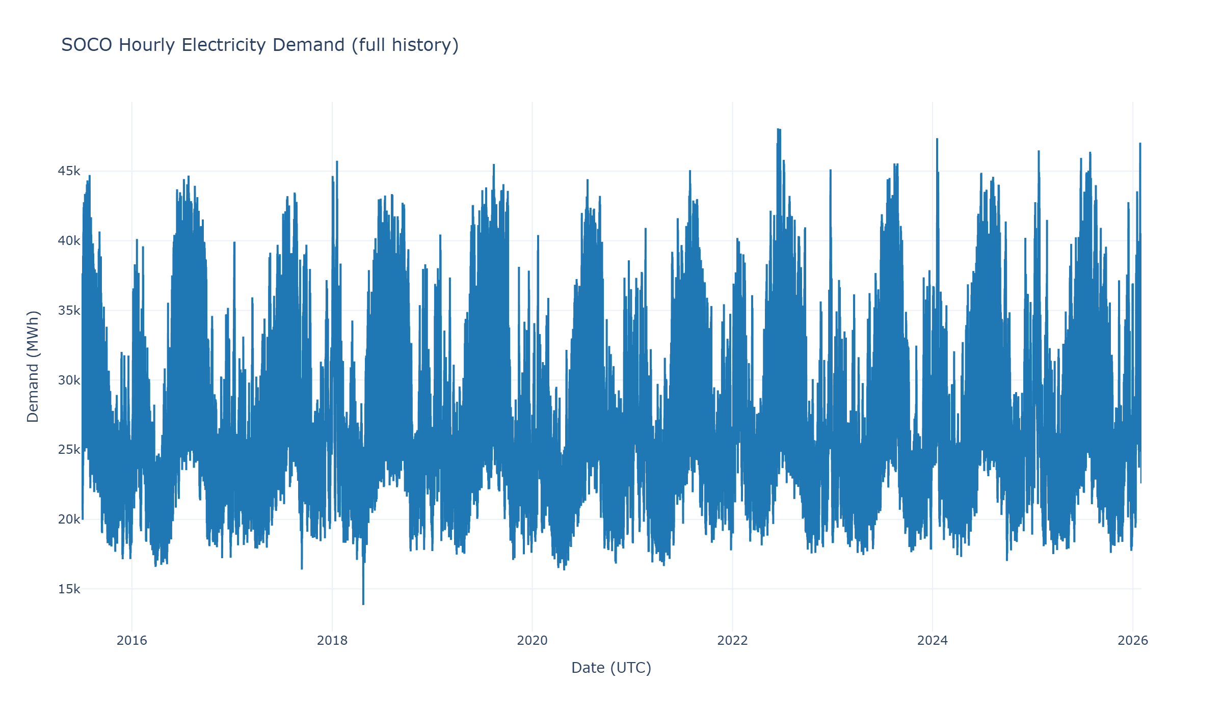
The target variable is demand_imputed_pudl_mwh, an hourly demand series for the SOCO balancing authority derived from PUDL/EIA-930 grid operations data. Weather features are integrated from regional Open-Meteo historical weather records, then transformed into modeling inputs that reflect both daily load shape and temperature-driven heating and cooling effects.
The final modeling dataset supports apples-to-apples model comparison by using consistent timestamps, aligned predictors, and time-aware train, validation, and test splits.
Feature Engineering
Feature engineering converts raw operations and weather data into horizon-safe predictors for hourly forecasting. The goal is to capture recurring load structure without allowing future demand information to leak into model training or evaluation.
- Lag features: recent demand history such as hourly, daily, and weekly lags that capture autocorrelation.
- Rolling-window statistics: shifted rolling means and variability metrics that summarize recent load behavior.
- Calendar encoding: hour-of-day, day-of-week, weekend, seasonal, and holiday-style effects.
- Weather integration: regional temperature, dew point, humidity, pressure, wind, precipitation, and radiation signals.
- Heating/cooling features: degree-hour style variables that represent nonlinear temperature-demand response.
- Pruned feature set: a simplified XGBoost Top-50 variant for comparing full-feature performance against a leaner model.
Modeling Approach
The revamped project compares four model configurations against the same target and evaluation split. SARIMAX acts as the demand-only statistical baseline, Prophet provides a flexible decomposable time-series model, and XGBoost models treat forecasting as a supervised regression problem with engineered demand, weather, and calendar features.
- SARIMAX: baseline statistical time-series model using historical demand structure.
- Prophet: time-series model with trend and seasonality components plus weather-aware regressors.
- XGBoost Full: supervised gradient-boosting model trained with the full engineered feature set.
- XGBoost Pruned Top-50: optimized XGBoost variant using a reduced set of the most useful features.
- Optuna tuning: model hyperparameters are optimized using reproducible search workflows.
- MLflow tracking: runs, parameters, metrics, predictions, and artifacts are logged for comparison and auditability.
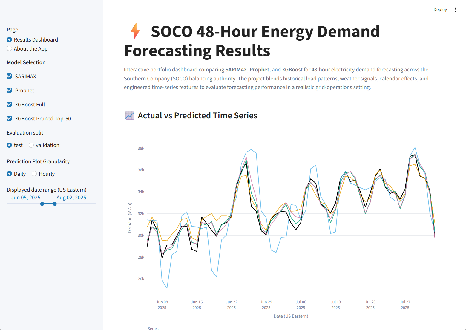
Interactive Results Dashboard
The Streamlit app was redesigned as an interactive results dashboard. It starts with the actual versus predicted time-series plot, supports model-selection controls, allows the user to switch between test and validation splits, and recalculates error metrics for the displayed date range.
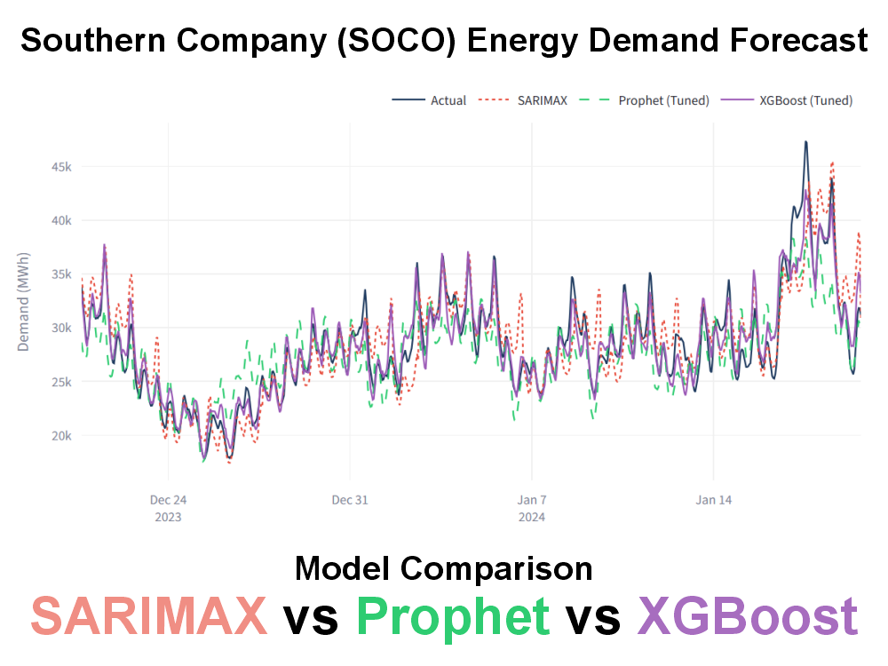
- Actual vs. predicted: daily or hourly forecast traces compare SARIMAX, Prophet, XGBoost Full, and XGBoost Pruned Top-50 against observed demand.
- Date-range filtering: the visible forecast window can be adjusted interactively from the dashboard sidebar.
- Metric cards: RMSE, MAE, and MAPE are recalculated for the selected time range and split.
- Deployment-friendly data: the deployed app reads static dashboard-ready files rather than training or tuning at runtime.
Forecast Evaluation & Model Comparison
Evaluation focuses on leakage-aware comparison across the same modeling data and consistent metrics. The dashboard stores standardized per-model result files so that full-test metrics, validation metrics, daily predictions, hourly predictions, horizon errors, feature importance, and SHAP summaries can be refreshed after new MLflow runs.
Model Comparison Framework
| Model | Primary Role | Input Signal | Dashboard Metrics |
|---|---|---|---|
| SARIMAX | Statistical baseline | Demand history | RMSE, MAE, MAPE, horizon errors |
| Prophet | Time-series + weather baseline | Trend, seasonality, calendar effects, weather regressors | RMSE, MAE, MAPE, horizon errors |
| XGBoost Full | Full supervised ML model | Demand lags, rolling statistics, weather, calendar, interaction features | RMSE, MAE, MAPE, feature importance, horizon errors |
| XGBoost Pruned Top-50 | Simplified high-signal ML model | Top retained predictors from the full feature set | RMSE, MAE, MAPE, feature importance, SHAP top features, horizon errors |
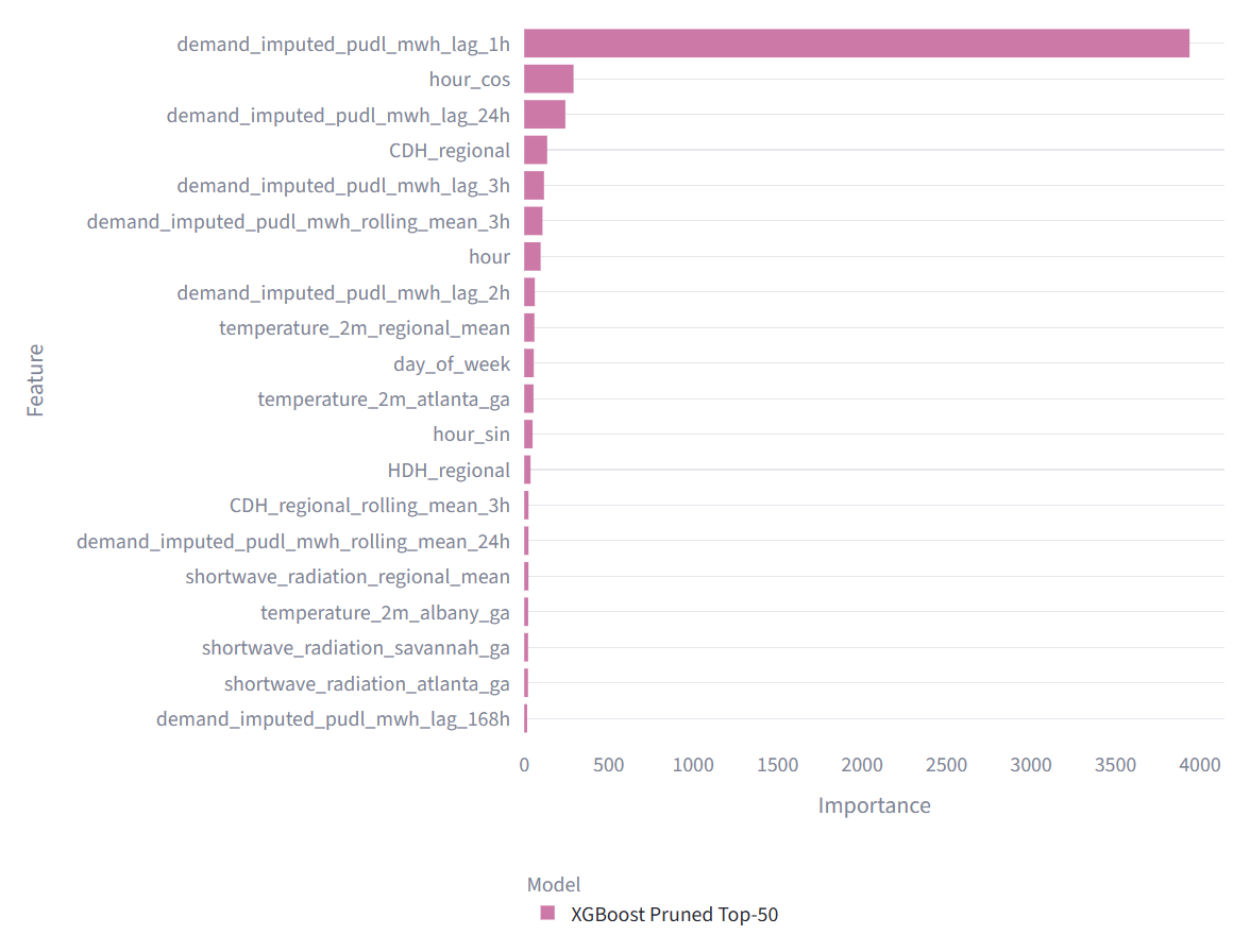
Interpretability: What Drives the Forecast?
The pruned XGBoost model highlights the dominant predictors behind short-term load forecasting. Recent demand history is the strongest signal, while calendar features and regional heating and cooling indicators add operational context for daily load shape and weather-sensitive demand.
- Recent load dominates: the most important feature is the one-hour lag of demand.
- Daily structure matters: 24-hour lags, hour encodings, and rolling windows capture repeating load cycles.
- Weather adds explanatory value: temperature and degree-hour features help represent HVAC-driven demand.
- Pruning supports communication: the Top-50 model is easier to explain while retaining the core demand, weather, and calendar signals.
Dashboard Data Architecture
The deployed dashboard uses a static model-results folder designed for fast loading on GitHub Pages and Streamlit Community Cloud. After new experiments are completed, the best SARIMAX, Prophet, XGBoost Full, and XGBoost Pruned runs are exported into standardized result files and committed with the app.
- model_comparison_metrics.csv: one-row-per-model summary metrics for dashboard cards and tables.
- manifest.json: model names and dashboard metadata.
- Per-model metrics.csv: model-specific evaluation metrics.
- predictions.csv and daily_predictions.csv: hourly and dashboard-friendly daily prediction files.
- horizon_errors.csv: forecast-error diagnostics by prediction horizon.
- feature_importance.csv and shap_top_features.csv: optional interpretability artifacts for tree-based models.
Operational & Portfolio Value
This project demonstrates how to move beyond a notebook-only forecast into a reproducible, reviewable, and stakeholder-friendly ML workflow for energy operations.
- Utility relevance: frames forecasting around day-ahead load planning, reserves, and grid-operations decisions.
- Fair comparison: evaluates multiple forecasting strategies on consistent data and splits.
- Leakage awareness: emphasizes time-aware splitting and horizon-safe feature engineering.
- Model interpretability: uses feature importance and SHAP summaries to explain why forecasts move.
- Production-minded packaging: separates offline training and tuning from lightweight dashboard deployment.
GitHub Repository & Live Demo
The full implementation and public dashboard are available through the links below.
🔗 View Project Repository on GitHub
The repository includes data preparation, feature engineering, model training and tuning, MLflow tracking outputs, static dashboard-ready model-result artifacts, Plotly figures, and the Streamlit portfolio app.